Servo Drive Tuning: PID Gains Explained
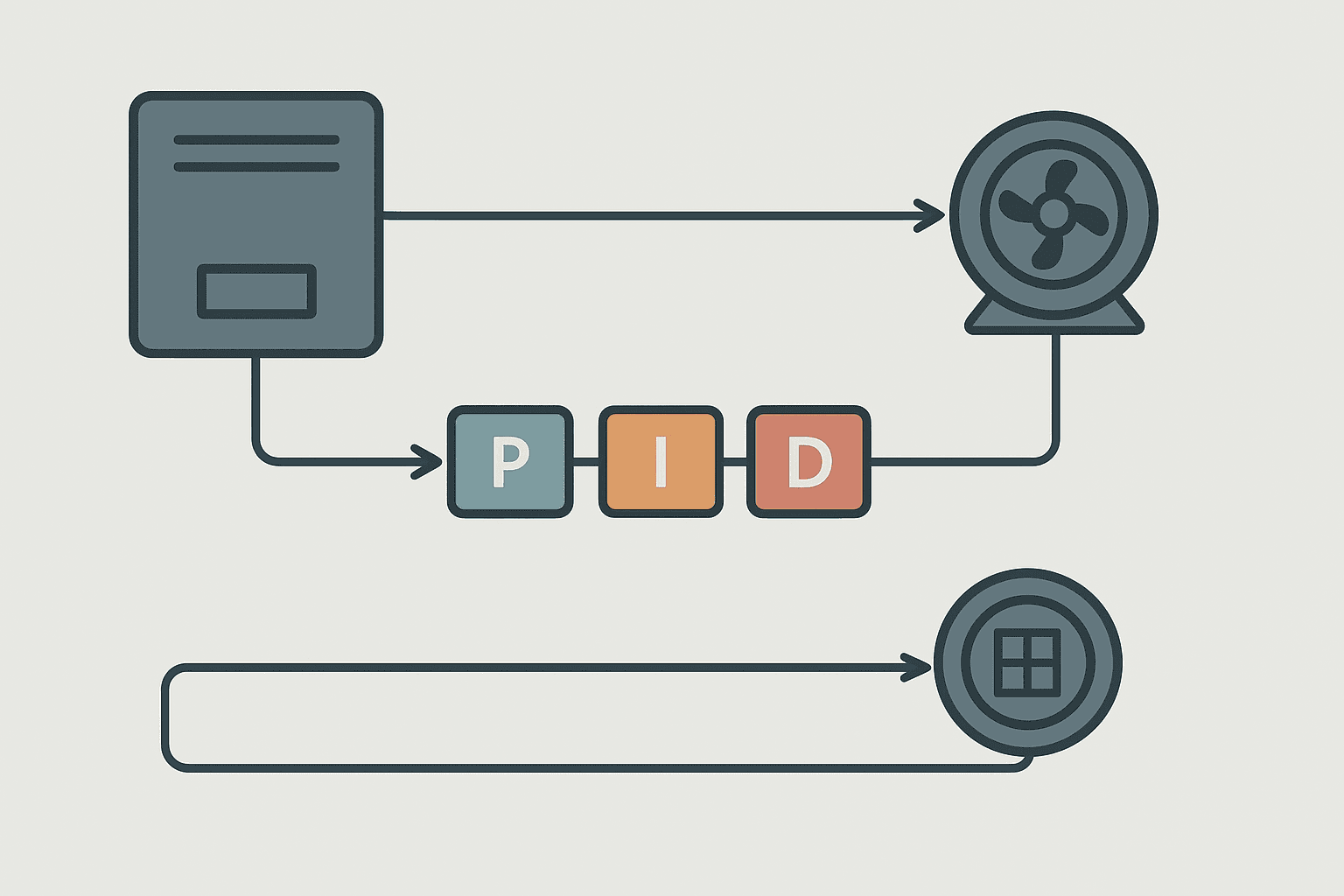
Most servo drives ship from the factory with autotuning routines that get you 80% of the way there. The remaining 20% is where your machine either runs beautifully or oscillates itself into a fault. To close that gap you need to understand what the three gains are actually doing, not just which direction to turn them.
Servo Drive Tuning: The Three Loops You Are Actually Tuning
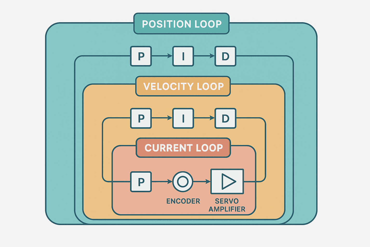
A typical servo drive runs three nested control loops, each one inside the other. From outermost to innermost: position loop, velocity loop, current (torque) loop. The current loop runs at the hardware level, usually 10 to 20 kHz, and you almost never touch it. The velocity loop runs at 1 to 4 kHz on most drives. The position loop is the outermost and slowest, often 500 Hz to 1 kHz. Each loop has its own P, I and sometimes D gains.
What Each PID Gain Does in a Servo Velocity Loop
Proportional Gain (Kp): The Muscle
Proportional gain multiplies the current velocity error (commanded speed minus actual speed) and outputs a torque demand directly proportional to that error. Double Kp and the drive pushes twice as hard for the same speed error. Higher Kp means faster response and stiffer feel. Push it too high and the motor starts to buzz, then oscillate, then trip on overcurrent or position error. On a Mitsubishi MR-J5 amplifier the velocity loop gain is called VG1 and ships at a default of 24 rad/s on most models. On a Siemens S120 it is the speed controller proportional gain Kp in the expert list.
Integral Gain (Ki): The Memory
Integral gain accumulates velocity error over time and adds it to the output. Its job is to eliminate steady-state error. If your motor is running at 1450 rpm instead of the commanded 1500 rpm, Kp alone can't zero that out because a zero error produces zero output. Ki keeps winding up the output until the error disappears. Too much Ki causes slow, low-frequency oscillation that looks like the motor hunting. On a Yaskawa Sigma-7 the velocity integral time constant Ti is the reciprocal of Ki, so a smaller Ti value means more aggressive integral action. This trips people up constantly.
Derivative Gain (Kd): The Damper
Derivative gain reacts to the rate of change of error. It sees the error getting worse quickly and applies a braking force before the overshoot happens. In servo drives, true velocity-loop derivative gain is rare because differentiating a noisy encoder signal amplifies noise badly. What you see instead is a velocity feedback filter (low-pass) and sometimes a feed-forward gain. The position loop usually has a derivative term, effectively acting on velocity error in the outer loop. On Rockwell Kinetix drives in Studio 5000, the position loop exposes Kp (position proportional) and optionally a velocity feed-forward percentage.
Practical Tuning Sequence: Velocity Loop First
Do not touch the position loop until the velocity loop is stable. Every experienced motion engineer I know works in this order:
- Set Ki (or Ti) to minimum so integral action is nearly off. You want to isolate proportional response.
- Increase Kp in 10-20% steps. After each step, command a velocity step (jog) and watch the response on the drive's oscilloscope or trace function. You are looking for clean response with less than 10% overshoot.
- When you see the first hint of ringing (the speed trace oscillates 2 to 3 times after a step), back Kp off by 20-30%. That is your working proportional gain.
- Now slowly increase Ki (or decrease Ti) until steady-state error drops to near zero. Watch for low-frequency hunting. A little overshoot on a step is acceptable. Sustained oscillation means you have gone too far.
- If the drive has a velocity feed-forward gain, add it now. This reduces following error during acceleration without affecting stability. Start at 80% and trim up.
- Once the velocity loop is settled, set position loop gain (Kpp). A common starting point is Kpp in rad/s = velocity loop bandwidth divided by 4 to 6. On a Mitsubishi MR-J5, if VG1 = 100 rad/s, start PG1 around 20 to 25 rad/s.
Reading the Oscilloscope Trace: What You Should See
Every modern servo amplifier has a built-in trace or oscilloscope function. On a Siemens S120 it is the STARTER/Startdrive trace. On a Yaskawa Sigma-7 it is SigmaWin+. On a Mitsubishi MR-J5 it is MR Configurator2. Use it. Looking at a motor with your eyes and listening to sound tells you some things, but the trace tells you everything.
| What you see on the trace | What it means | What to adjust |
|---|---|---|
| Slow approach, no overshoot, lots of steady-state error | Kp too low, Ki too low | Increase Kp first, then Ki |
| Fast response, 5-15% overshoot, settles cleanly | Well tuned velocity loop | Leave it, move to position loop |
| High-frequency buzz or ripple on speed trace | Kp too high, mechanical resonance | Reduce Kp, add a notch filter at resonant frequency |
| Slow oscillation, 1-5 Hz hunting | Ki too high (or Ti too small) | Reduce Ki / increase Ti |
| Following error grows during acceleration, settles at rest | Velocity feed-forward too low | Increase Vff gain |
| Position overshoot on every move, then oscillation | Position loop Kpp too high | Reduce Kpp by 20% |
Notch Filters: When the Machine Has Resonance
Resonance is the enemy of high Kp. Every mechanical assembly has a natural frequency where it wants to ring. A ball screw and carriage might resonate at 200 Hz. A long belt drive might resonate at 40 Hz. When your Kp is high enough to excite that frequency, you get a sustained buzz that can shake bolts loose and eventually damage the drive or the encoder. The fix is a notch filter centred on the resonant frequency, not a lower Kp.
To find the resonant frequency: use the frequency sweep or FFT function in the drive software. On a Yaskawa Sigma-7, SigmaWin+ has a 'mechanical analysis' function that sweeps the axis and plots the frequency response. On a Mitsubishi MR-J5, the adaptive vibration suppression filter can detect and set notches automatically. On a Siemens S120, you run the speed controller optimization in Startdrive and it identifies resonant frequencies and suggests filter settings. Once you have a notch at the right frequency you can push Kp 30-60% higher than before.
Load Inertia Ratio: The Number That Sets Your Starting Point
Before you even start tuning, calculate your load inertia ratio. This is the total reflected inertia of the load at the motor shaft divided by the motor rotor inertia. A 1:1 ratio is easy to tune. A 10:1 ratio is manageable with care. Above 30:1 you are fighting the physics and need a gearbox or a bigger motor.
Most servo drive sizing software (Siemens SIZER, Yaskawa DriveWizard, Mitsubishi Servo Sizer) will calculate this if you enter the load geometry. Do it before you buy the motor, not after. I have seen projects where someone picked a motor that was 'powerful enough' in torque but had a 50:1 inertia mismatch. The axis never tuned properly and they ended up replacing the motor with a larger frame just for the rotor inertia.
Autotuning: What It Actually Does and When to Trust It
Autotuning on a modern drive (Yaskawa Sigma-7 adaptive tuning, Mitsubishi MR-J5 one-touch tuning, Siemens S120 speed controller optimization) works by commanding a series of velocity steps or frequency sweeps, measuring the response, and calculating gains. It works well when the load is consistent, the coupling is stiff and the inertia ratio is below about 10:1. It struggles when the load changes during operation (a robot arm at different extensions, a conveyor that fills up with product), when the coupling is compliant (long belt, flexible shaft) or when you need very high bandwidth.
Use autotuning as a starting point, not a final answer. After autotuning, always run a step response trace and check the settling time and overshoot against your application requirements. For a pick-and-place machine needing 5 ms settling, the autotuned gains might be conservative. For a grinding spindle where vibration damages the workpiece, they might be too aggressive.
Connecting Servo Tuning Back to the PLC
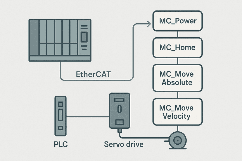
The PLC sees a servo axis through a motion controller or via the PLCopen function blocks covered in PLCopen Motion Blocks: MC_MoveAbsolute and Friends. From the PLC side, following error and actual velocity are the two signals that tell you whether your tuning is working. If following error on an MC_MoveAbsolute command is consistently above your tolerance, the velocity loop gains are too low or feed-forward is missing. If you see the axis overshoot and the position error goes briefly negative after a move, Kpp is too high relative to the velocity loop bandwidth.
On a Rockwell Kinetix 5700 with a Logix controller, you can monitor Axis.FollowingError, Axis.ActualVelocity and Axis.ActualTorque directly in the tag browser in Studio 5000. Set up a trend in Logix Designer and log a full move profile. You will see exactly where the following error peaks (usually during acceleration) and where it settles. That data tells you whether to adjust Vff, Kp or Ki.
A Realistic Tuning Target by Application
| Application | Typical velocity loop bandwidth | Following error tolerance | Key concern |
|---|---|---|---|
| General conveyor positioning | 50-150 rad/s | 1-5 mm | Smooth acceleration, no oscillation |
| Pick and place (high speed) | 200-400 rad/s | 0.1-0.5 mm | Fast settling, low inertia ratio needed |
| CNC milling axis | 300-600 rad/s | 0.01-0.1 mm | Stiffness, notch filters for chatter |
| Grinding spindle | 100-200 rad/s | N/A (velocity control) | Minimal vibration, smooth torque |
| Robot joint (payload varies) | 150-300 rad/s | 0.05-0.5 mm | Gain scheduling or adaptive tuning |
These are ballpark figures. Your actual targets come from the machine specification and the tolerance your process requires. Always document the final gain values and the trace screenshots in the commissioning record. When the machine needs a motor replacement six months later, those numbers save hours of re-tuning.
Frequently asked questions
What is the difference between velocity loop gain and position loop gain on a servo drive?
How do I know if my servo drive Kp is too high?
Why does my servo axis hunt slowly even though there is no high-frequency buzz?
Should I use autotuning or manual tuning for a servo drive?
What load inertia ratio is acceptable for a servo motor?
How do I monitor servo following error from the PLC?
Learn this by building it
There is a PLC in this site. It runs a real scan engine, checks your logic against the same tests a working machine would fail, and needs no download and no account.
Open the exercisesFree, no signup, runs in your browser. See all 16 exercises.
Was this helpful?