SCADA Historian: How Process Data Gets Logged
Most engineers treat the SCADA historian as an afterthought: the thing that makes trend screens work. That thinking leads to full disks, corrupted archives, and the angry phone call when someone asks for six months of reactor temperature data and you have three days. The historian is actually one of the most architecturally important pieces of a SCADA system, and it works very differently from what most people assume.
What a SCADA Historian Actually Is
A process historian is a purpose-built time-series database that records the value of plant tags at high speed and stores them efficiently over months or years. It is not a general-purpose SQL database. It is not the SCADA server's internal memory. And it is not the same as the live tag table you see on an operator display.
The distinction matters because time-series data has a very specific shape: millions of small (timestamp, value, quality) tuples arriving at rates anywhere from once per second to 100 Hz on fast analog loops. A relational database can store that, but the query performance and storage overhead become painful fast. Historians use compression algorithms and binary file formats tuned for exactly this pattern.
Common commercial historians include OSIsoft PI (now AVEVA PI System), Ignition's built-in Tag Historian (SQLite or external DB), Inductive Automation's reporting module, Wonderware Historian (AVEVA), Kepware ThingWorx Kepware Server with logging, and open-source options like InfluxDB or TimescaleDB. Each handles compression, retrieval and redundancy differently.
How SCADA Historian Data Logging Works Step by Step
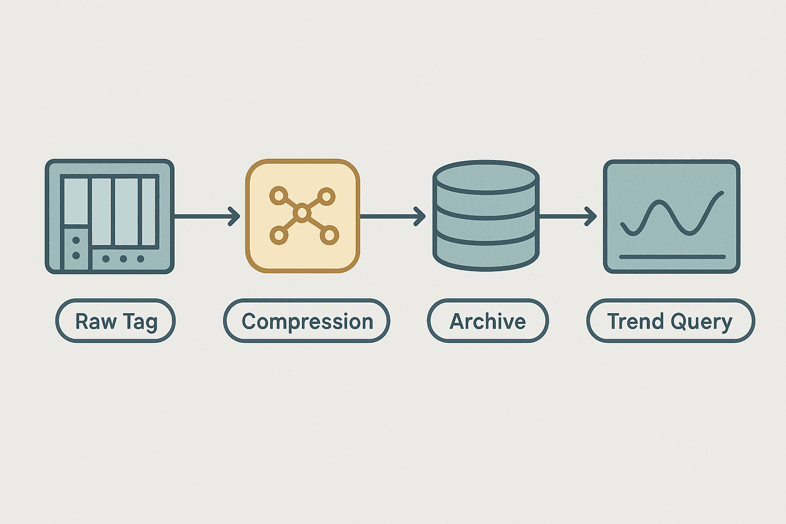
The data path from a field instrument to a historian query has several distinct stages. Understanding each one tells you where data can be lost, delayed or distorted.
- Tag scan: The SCADA server (or OPC server) polls the PLC or RTU at a configured scan rate, typically 1 s for process values and 100 ms for discrete alarms. The raw value lands in the live tag database.
- Deadband filtering: Before the historian writes anything, it checks whether the new value has changed enough to be worth recording. A flow tag with a 0.5% deadband on a 0-1000 L/min span will only generate a record if the reading moves more than 5 L/min from the last stored value. This alone can cut storage by 80% on a stable process.
- Exception reporting: Only changes that exceed the deadband are forwarded to the historian engine. This is sometimes called exception-based recording (EBR) and it is the core of why historians stay manageable.
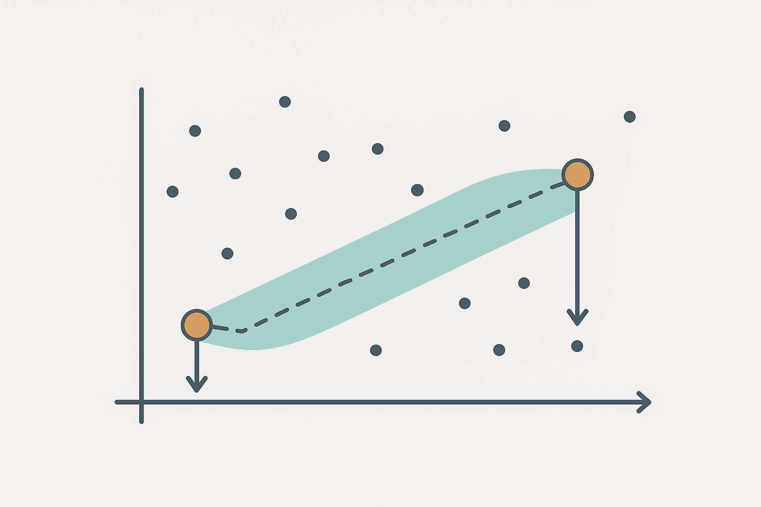
- Compression (swinging door): The most common algorithm used in historians like PI is swinging-door compression. Instead of storing every sampled point, it fits straight-line segments through the data. Points that fall within a compression deviation (e.g. 0.1% of span) of the extrapolated line are dropped. Only the points that break the line are archived.
- Archive storage: Compressed records go into the archive, a binary flat file or proprietary structure on disk. PI uses .arc files of fixed size (default 512 MB) that roll over on a schedule. Ignition writes to a configured SQL table or a dedicated file store.
- Retrieval and interpolation: When a trend query asks for data at a resolution finer than what was archived, the historian interpolates between stored points. This is transparent to the user but means a trend at 1-second resolution may contain calculated values, not raw samples.
Swinging Door Compression: The Numbers
It helps to put real numbers on compression. A 4-20 mA temperature tag scanned every 1 second on a slow thermal process might only generate 2 to 5 stored events per hour with typical compression settings. That is a 720x to 1800x reduction from raw samples. A fast pressure loop on a reciprocating compressor scanned at 100 ms might generate 200 events per minute even with compression, because the signal genuinely oscillates.
| Tag type | Scan rate | Compression deviation | Typical stored events/hr |
|---|---|---|---|
| Slow temperature (tank) | 1 s | 0.2% of span | 2-10 |
| Level (stirred vessel) | 1 s | 0.1% of span | 20-60 |
| Flow (liquid, stable) | 500 ms | 0.5% of span | 30-100 |
| Pressure (compressor) | 100 ms | 0.05% of span | 500-3000 |
| Discrete (motor run) | 100 ms | on-change only | varies by starts/stops |
Tag Configuration: What You Actually Have to Set
Whether you are using PI System, Ignition, or a simpler built-in historian, the same core parameters come up every time.
- Scan class / collection rate: How often the historian engine reads the source tag. Keep this at or above the PLC scan rate for the tag. There is no benefit going faster than the source updates.
- Exception deviation: The minimum change (in engineering units or percent of span) that triggers an exception record. Set too wide and you miss real process changes. Set to zero and you store every scan.
- Compression deviation: The maximum error allowed by the swinging-door algorithm. Typically set to the same value as exception deviation or slightly larger.
- Compression maximum time: The longest gap allowed between stored records even if the value has not changed. Common setting is 8 hours. Without this, a flat signal could have no stored point for days, which makes trend queries return nothing.
- Engineering units and span: Needed for percent-based deviation calculations and for sensible display on trends.
- Data type: Integer vs float vs string vs discrete (Boolean). Discrete tags use on-change recording with no compression.
Historian vs SCADA Live Tag Database: The Real Difference
The live tag database (sometimes called the real-time database or RTDB) holds the current value of every tag in memory. It is updated every scan cycle and has no history. When you look at a process value on an operator display, you are reading the RTDB.
The historian takes a feed from the RTDB and writes compressed snapshots to disk. When a trend screen asks for the last 8 hours of a tag, it is querying the historian archive, not the RTDB. This means the trend screen can show data from before the SCADA server was restarted, from before a network outage, or from last Tuesday at 3 AM when you were asleep.
Storage Sizing: How Much Disk Do You Actually Need
A very rough rule: a compressed float tag storing at an average of 100 events per hour uses about 1.5 to 2 KB per hour of archive. Scale that up:
- 1,000 tags at 100 events/hr average = 100,000 events/hr = roughly 150 MB/hr = 1.3 TB/year.
- Same 1,000 tags on a stable process at 10 events/hr average = 13 GB/year.
- Discrete tags (on-change) add very little unless the machine is cycling thousands of times per hour.
The range is huge because it depends entirely on process variability and compression settings. Measure your actual event rates in the first week of operation and project from there. Do not trust vendor estimates without knowing your specific process.
Querying Historian Data: Retrieval Modes
Most historians offer several retrieval modes and picking the wrong one gives you misleading trends.
| Retrieval mode | What it returns | Use it when |
|---|---|---|
| Interpolated | Values at evenly spaced timestamps, filled by linear interpolation | Trend displays, most dashboards |
| Recorded (raw) | Only the actual stored archive events | Audits, debugging compression settings, exact event times |
| Compressed | Archive events plus the current live value | Exporting data to a spreadsheet or MES |
| Plot (Ramp) | Alternating min/max values per display pixel | Dense trend displays to show true range without aliasing |
| Sampled | The value at the nearest archive point to each requested timestamp | Reporting at fixed intervals where interpolation would be misleading |
Open-Source Options: InfluxDB and TimescaleDB
If you are working on a smaller project or a greenfield IIoT system, purpose-built open-source time-series databases are worth knowing. InfluxDB uses a line protocol for writes and Flux or InfluxQL for queries. It has built-in downsampling tasks that approximate swinging-door compression. TimescaleDB sits on top of PostgreSQL, which means your existing SQL skills transfer directly.
Neither has the decades of historian-specific features that PI or Wonderware carry, but for a 500-tag system with a small budget they are completely viable. Ignition's built-in Tag Historian can also write to either via JDBC or the Cirrus Link MQTT modules, which makes them practical in real production environments.
Common Historian Mistakes and How to Avoid Them
- Logging every tag at the same rate. A motor run status does not need a 100 ms scan class. Assign scan classes deliberately based on how fast the value actually changes.
- Zero compression deviation on all tags. Copying a tag configuration template with compression disabled means you store every scan point. Disk fills in weeks instead of years.
- No maximum time setting. A stable tank level with a wide deadband can go hours without a stored event. Set a maximum time (4 to 8 hours is typical) so trends do not show gaps.
- No store-and-forward. Any network maintenance window becomes a permanent hole in the archive.
- Mixing historian and SQL reporting queries. Running complex SQL joins against a historian's internal tables can lock write threads. Use the historian's own API or OPC UA HA for reads.
- Not backing up the archive separately from the OS. If the historian server disk fails and the archive is on the same volume, you lose both. Keep archives on a separate volume or NAS.
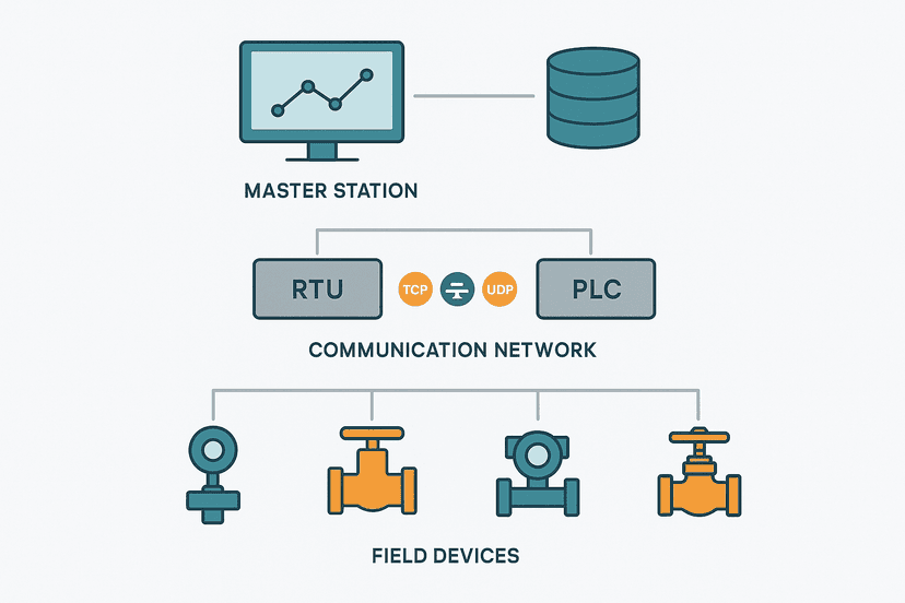
For broader context on how the historian fits into the full SCADA architecture, SCADA System Architecture: Layers, RTUs and the Master Station covers how data flows from the field level up through the control network to where the historian lives.
Frequently asked questions
What is the difference between a SCADA historian and a regular database?
How does swinging-door compression work in a SCADA historian?
What is store-and-forward in a process historian?
Can I use InfluxDB as a SCADA historian?
Why does my historian trend look different from the live process value?
How much disk space does a SCADA historian need?
Learn this by building it
There is a PLC in this site. It runs a real scan engine, checks your logic against the same tests a working machine would fail, and needs no download and no account.
Open the exercisesFree, no signup, runs in your browser. See all 16 exercises.
Was this helpful?