What is a PLC scan cycle?

The PLC scan cycle is the repeating sequence a PLC executes continuously: read all physical inputs into memory, execute the user program against that memory snapshot, write the results to physical outputs, then perform housekeeping. This cycle repeats hundreds of times per second in a normal control system.

How long does a PLC scan cycle take?

Typical scan times range from 1 ms to 20 ms for most industrial PLCs. A small Siemens S7-1200 or Rockwell Micro820 with a few hundred rungs usually scans in 2 to 5 ms. Large programs with heavy math, string handling, or many function blocks can push past 50 ms on older hardware.

Why does the PLC read inputs only once per scan?

The PLC copies all physical input states into an input image table at the start of each scan. This snapshot keeps input values consistent throughout the whole program, so a bit that changes mid-scan does not cause unpredictable behaviour in different rungs. The new state appears at the start of the next scan.

What happens if the PLC scan time exceeds the watchdog timer?

If a scan takes longer than the configured watchdog timeout, typically 100 to 500 ms, the CPU goes to fault mode, outputs drop to their configured safe states, and a diagnostic fault is logged. This protects the machine from a frozen program. You must clear the fault and restart the CPU to resume.

Can a PLC miss a fast input signal between scans?

Yes. A pulse shorter than one full scan cycle can be missed entirely because inputs are only sampled once per scan. High-speed counting or capture inputs use hardware latching, interrupt routines, or dedicated high-speed counter modules to catch signals faster than the main scan allows.

What is the difference between scan time and cycle time?

Scan time and cycle time are often used interchangeably. Technically, cycle time includes all four phases: input scan, program execution, output scan, and housekeeping. The program execution phase usually dominates, but on larger systems the I/O update and communications overhead can add several milliseconds.

What is the PLC image table?

The image table (also called the process image or I/O table) is a block of PLC memory that holds a copy of all input and output states. The CPU reads physical inputs into the input image at scan start, executes logic against it, and copies output image results to physical outputs at scan end.

How do I check the scan time on my PLC?

Most PLCs expose scan time diagnostics in their programming software. In TIA Portal, check the CPU's online diagnostics under cycle time. In Studio 5000, use the Controller Properties diagnostics tab. On Omron Sysmac, the Task Monitor shows cycle time per task. All three also show minimum, maximum, and current values.

Does adding more ladder rungs always increase scan time?

Yes, but the relationship is not always linear. Simple XIC/XIO contact rungs add microseconds each. Heavy instructions like PID, string operations, or large array moves add far more. Communications handled in the scan rather than a background task can also spike cycle time unpredictably.

What is a periodic task or timed interrupt, and how does it differ from the main scan?

A periodic task interrupts the main scan at a fixed interval, for example every 10 ms, to run time-critical logic independently of the main program length. This is common for PID loops and motion control. The main scan continues when the interrupt finishes. Overloading periodic tasks causes scan overruns.

How the PLC Scan Cycle Works: Step by Step

‌

Flat vector infographic of the PLC scan cycle showing four phases arranged in a circle: input scan, program execution, output scan, and housekeeping with connecting arrows

Every PLC program you write runs inside a loop. Not a loop you coded, but the hardware loop the CPU runs automatically, over and over, for as long as the PLC is powered. That loop is the scan cycle, and understanding exactly what it does in each phase is the single most important concept in PLC programming. Get this wrong and your logic will behave in ways that seem impossible until you understand the timing.

What Is the PLC Scan Cycle?

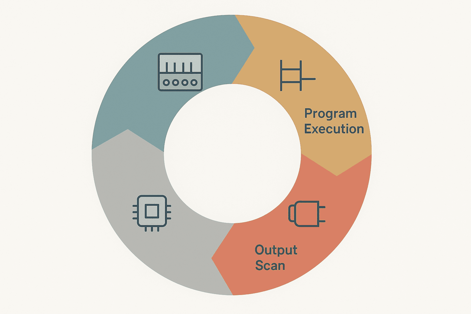
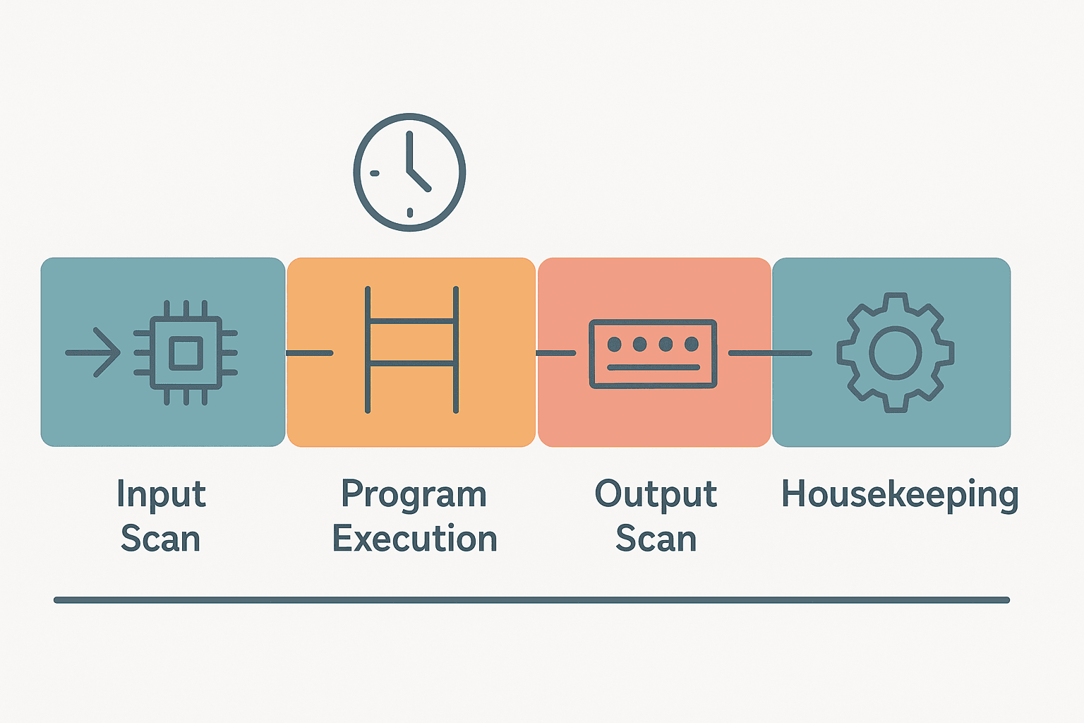
The PLC scan cycle is the continuous, repeating sequence a programmable logic controller executes to read physical inputs, run the user program, and drive physical outputs. Each complete pass through this sequence is one scan. A typical industrial PLC completes 50 to 500 scans per second, with each scan taking roughly 1 to 20 ms depending on program size and hardware. The cycle has four distinct phases: input scan, program execution, output scan, and housekeeping.

The Four Phases of the PLC Scan Cycle

Phase 1: Input Scan

At the very start of each scan, the CPU reads every physical input channel, whether 24 VDC digital inputs, analog channels, or discrete safety inputs, and copies their states into a dedicated block of memory called the input image table (Siemens calls it the Process Image Input, or PII; Rockwell calls it the input data table; the concept is identical everywhere). That snapshot is frozen for the rest of the scan. If a sensor changes state halfway through program execution, the PLC does not see it until the next scan's input phase.

This is not a limitation, it is a deliberate design choice. A consistent input snapshot means that every rung in your program sees the same input values. Without it, a single sensor changing mid-scan could give rung 5 and rung 500 contradictory information, causing logic that is impossible to debug. The snapshot makes behavior deterministic.

Short-pulse problem: If a physical input goes high and returns low within a single scan period, the PLC may never see it at all. On a 10 ms scan, any pulse shorter than 10 ms is at risk. For fast signals like encoder pulses or reject triggers, use a hardware-latching high-speed input or a dedicated counter module. See the discussion on input pulse stretching and counter instructions for ladder workarounds.

Phase 2: Program Execution

The CPU now executes your program from the first rung to the last, evaluating each instruction against the input image table and internal memory bits. When a rung's logic evaluates true and drives an output coil, the CPU writes that result to the output image table, another block of memory. It does not yet change anything on the physical output terminals. Everything stays in memory until Phase 3.

This phase is where almost all your application logic lives: interlocks, timers, counters, PID loops, sequencers, analog scaling. The time it takes depends almost entirely on how much code you have and how complex the instructions are. A few hundred simple ladder rungs might take 1 ms. A large program with floating-point math, string handling, and hundreds of function blocks on an older CPU can take 30 ms or more. Understanding PLC memory and addressing helps you write leaner, faster programs.

One subtlety that trips up newer engineers: because the CPU scans top to bottom in a single pass, a coil that gets set on rung 10 is immediately visible to rung 11 in the same scan, because the CPU reads the output image table for internal bits. But a physical input change on that same rung 10 result won't be visible until the next scan's input phase. This difference between internal memory and physical I/O is the source of a lot of confusing behaviour on first projects. If you want to understand contacts in depth, XIC vs XIO contacts explained covers exactly how the CPU evaluates each one.

Phase 3: Output Scan

Once program execution finishes, the CPU copies the output image table to the physical output terminals. Every relay, transistor, or triac output module gets updated in one pass. This is when your valve actually energises, your motor contactor actually closes, and your indicator light actually turns on. The physical world only changes during this phase.

On remote I/O systems over networks like PROFINET or EtherNet/IP, this phase also involves sending updated output data to remote I/O nodes and waiting for acknowledgement. That network latency adds to your effective cycle time. A local I/O update might take 0.1 ms; a remote node over EtherNet/IP can add 1 to 4 ms depending on packet scheduling.

Phase 4: Housekeeping

After the outputs are updated, the CPU performs housekeeping: servicing the watchdog timer, processing communications requests from programming software or HMIs, handling background tasks, updating diagnostic buffers, and managing any interrupt tasks that are queued. This phase is often invisible to the programmer but it matters. Heavy communications load, lots of connected HMI clients, or a chatty OPC UA server can significantly extend the housekeeping phase and inflate your scan time.

Flat vector timeline diagram of the four PLC scan cycle phases showing input scan feeding a memory image table, program execution against that image, output scan writing to physical terminals, and a housekeeping phase with a CPU icon — The four phases of the PLC scan cycle. Program execution dominates scan time in most applications.

Real Scan Times: What to Expect

PLC Platform	Typical Scan Time	Notes
Siemens S7-1200	1 to 5 ms	Scales with OB1 program size; comms add overhead
Siemens S7-1500	0.5 to 3 ms	Faster CPU, bit operations 60x quicker than 1200
Rockwell CompactLogix	2 to 8 ms	Continuous task; periodic tasks run independently
Omron NX1P2 (Sysmac)	1 to 4 ms	Primary periodic task, default 4 ms period
Mitsubishi iQ-R	0.98 to 5 ms	High-speed scanning mode available on some CPUs
Beckhoff TwinCAT 3	0.1 to 1 ms	Real-time kernel; hard real-time at 250 µs possible

Indicative scan times for common platforms under light to moderate loads. Always measure on your actual hardware.

These numbers assume a reasonably sized program. If you start adding heavy floating-point math, large UDT arrays, or complex function blocks, scan time climbs fast. I once saw a Rockwell CompactLogix on a packaging line hit 45 ms because someone had dropped a large string-processing routine into the main continuous task instead of a background task. The machine started missing short product-detect pulses and the cause took two hours to find.

The Watchdog Timer: Your Safety Net

Every PLC has a watchdog timer. At the start of each scan, the watchdog is reset. If the scan completes normally before the watchdog expires, all is well. If a bug, an infinite loop, or a heavily overloaded CPU causes the scan to run past the watchdog timeout (typically configurable from 100 ms to 500 ms), the CPU trips to fault mode, all outputs go to their configured safe states (usually de-energised), and a fault is logged. This is a deliberate safety mechanism, not a bug. You can read more about diagnosing the CPU fault that follows in PLC CPU faults: how to diagnose them step by step.

Periodic Tasks and Interrupt Routines

Most modern PLCs support more than just the main cyclic scan. Periodic tasks run at a fixed time interval regardless of main scan length. You might put a PID loop in a 10 ms periodic task so it executes at a consistent rate even if the main scan varies between 5 and 15 ms. Event-driven interrupt routines fire on a rising edge of a specific input, instantly interrupting the main scan, running their code, then returning. These are essential for catching fast signals that the main scan would miss.

Siemens uses Organisation Blocks (OBs) for this: OB1 is the main cyclic scan, OB30 through OB38 are time-of-day interrupt OBs, and OB40 is a hardware interrupt OB. Rockwell uses Continuous, Periodic, and Event tasks in Studio 5000. Omron Sysmac uses Primary, Periodic, and Event tasks. The concept is the same across all of them.

Field tip: Keep your main scan lean. Move heavy math, communications polling, and reporting logic into lower-priority periodic tasks. Your control-critical logic in the main scan stays fast and predictable. This is exactly what PLC scan cycle troubleshooting recommends when tracking down timing-related faults.

How the Scan Cycle Affects Your Logic

Understanding the scan cycle changes how you write programs. A few practical consequences:

One-shot instructions matter: Rising-edge (OSR) and falling-edge (OSF) instructions detect the transition between scans, not within a scan. They produce a one-scan-wide pulse when a bit changes state. This is critical for incrementing counters or latching alarms correctly. See PLC internal bits: flags and coils for how these work in practice.
Timer accuracy is limited by scan time: A TON timer accumulates time in scan-sized increments. If your scan is 10 ms, your timer resolution is approximately 10 ms. For a 10-second setpoint that is fine. For a 50 ms setpoint, the error is significant.
Output feedback takes at least one scan: If you turn on an output and check a feedback input in the same scan, the feedback bit will not have updated yet. It reflects the state at the start of that scan. Your feedback check belongs in the next rung after a minimum delay or in the following scan.
Rung order matters for internal bits: A coil set on rung 50 is visible to rung 51 in the same scan. This is different from physical outputs, which don't update until the output scan phase. Design your program so rungs that depend on each other are in the right order.
Avoid long blocking operations in the main scan: File operations, large array copies, and certain communications instructions can hold up the main scan for many milliseconds. Use asynchronous or background task alternatives where available.

Checking Scan Time in Your Programming Software

Every major platform exposes scan time diagnostics. In TIA Portal, go online to your S7-1200 or S7-1500 and open the CPU's online diagnostics. The Cycle Time section shows minimum, maximum, and current cycle time in milliseconds. If you see the maximum value climbing over time, something in your program is occasionally taking much longer than average, and that is worth investigating. The S7-1200 first program guide walks through getting online and reading these diagnostics for the first time.

In Studio 5000, right-click the controller in the I/O tree and select Properties, then the General tab. The controller diagnostics show current, maximum, and minimum scan times. In Omron Sysmac Studio, the Task Monitor under the Controller tab shows execution time per task. In GX Works3 for Mitsubishi, the diagnostics menu shows scan time and any watchdog overruns.

If you are seeing PLC scan cycle problems or timing faults, measuring the scan time trend over time (not just a snapshot) is the first step. A scan that is consistently 8 ms but occasionally spikes to 80 ms tells a very different story than one that has steadily grown from 5 ms to 40 ms over six months of feature additions.

How the Scan Cycle Connects to the Wider System

The scan cycle does not exist in isolation. The PLC is connected to sensors, drives, HMIs, and other controllers. Every one of those connections has its own timing. A 4-20 mA analog input is sampled once per scan (or at a hardware rate that is then synchronised to the scan). A VFD receiving a speed reference over EtherNet/IP gets updated at the network's scheduled rate, which may or may not align with your scan. An HMI reading tag values polls the PLC at its own update rate, typically 500 ms to 1 second, much slower than the scan.

Understanding that all of these rates are different, and that the scan cycle is the fastest and most fundamental of them, helps you design systems that behave predictably. Fast safety logic belongs in the PLC scan or a high-priority interrupt task. Trend logging belongs in the historian, not in a PLC rung that runs every 5 ms.

The PLC also coordinates with SCADA and supervisory systems. The scan cycle is the source of all the real-time data that SCADA systems consume, but SCADA operates at a much coarser time scale. Knowing the difference prevents you from over-engineering the PLC side to compensate for something better handled at the SCADA layer.

Keep Learning

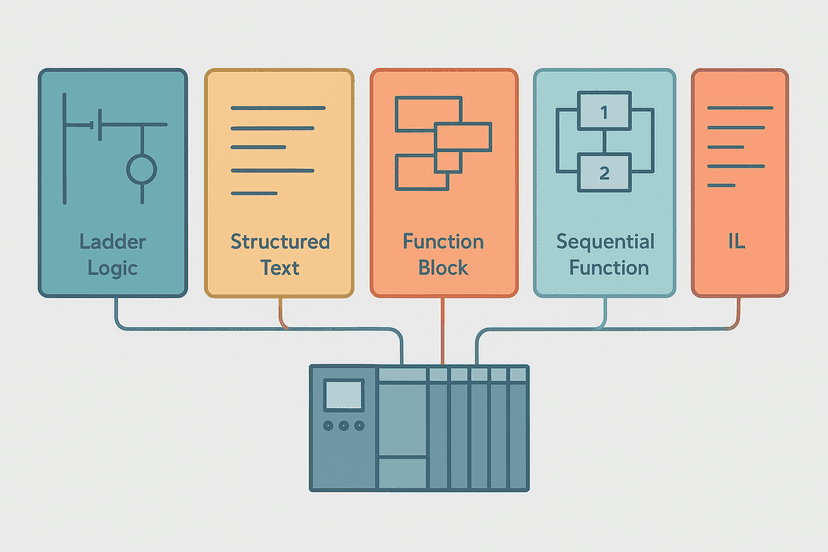
The scan cycle is the foundation everything else builds on. Once it clicks, ladder logic, timers, and counters all make more sense. A good next step is to see scan-related timing in action through PLC scan cycle troubleshooting: logic and timing faults, then reinforce the programming fundamentals in 5 types of PLC programming languages explained. If you want to understand how the CPU manages data alongside the scan, PLC memory and addressing explained fills in the rest of the picture.